Custom Epiworkflows

If you want to do custom data preprocessing or fit a model that isn’t included in the canned workflows, you’ll need to write a custom epi_workflow().

To get understand how to work with custom epi_workflow()s, let’s recreate and then modify the four_week_ahead example from the landing page. Let’s first remind ourselves how to use a simple canned workflow:

training_data <- covid_case_death_rates |>
  filter(time_value <= forecast_date, geo_value %in% used_locations)
four_week_ahead <- arx_forecaster(
  training_data,
  outcome = "death_rate",
  predictors = c("case_rate", "death_rate"),
  args_list = arx_args_list(
    lags = list(c(0, 1, 2, 3, 7, 14), c(0, 7, 14)),
    ahead = 4 * 7,
    quantile_levels = c(0.1, 0.25, 0.5, 0.75, 0.9)
  )
)
four_week_ahead$epi_workflow
#> 
#> ══ Epi Workflow [trained] ═══════════════════════════════════════════════════
#> Preprocessor: Recipe
#> Model: linear_reg()
#> Postprocessor: Frosting
#> 
#> ── Preprocessor ─────────────────────────────────────────────────────────────
#> 
#> 7 Recipe steps.
#> 1. step_epi_lag()
#> 2. step_epi_lag()
#> 3. step_epi_ahead()
#> 4. step_naomit()
#> 5. step_naomit()
#> 6. step_training_window()
#> 7. check_enough_data()
#> 
#> ── Model ────────────────────────────────────────────────────────────────────
#> 
#> Call:
#> stats::lm(formula = ..y ~ ., data = data)
#> 
#> Coefficients:
#>       (Intercept)    lag_0_case_rate    lag_1_case_rate    lag_2_case_rate  
#>        -0.0060191          0.0004648          0.0021793          0.0004928  
#>   lag_3_case_rate    lag_7_case_rate   lag_14_case_rate   lag_0_death_rate  
#>         0.0007806         -0.0021676          0.0018002          0.4258788  
#>  lag_7_death_rate  lag_14_death_rate  
#>         0.1632748         -0.1584456
#> 
#> ── Postprocessor ────────────────────────────────────────────────────────────
#> 
#> 5 Frosting layers.
#> 1. layer_predict()
#> 2. layer_residual_quantiles()
#> 3. layer_add_forecast_date()
#> 4. layer_add_target_date()
#> 5. layer_threshold()
#>

Anatomy of an `epi_workflow`

An epi_workflow() is an extension of a workflows::workflow() that handles panel data and post-processing. All epi_workflows, including simple and canned workflows, consist of 3 components.

Preprocessor

A preprocessor transforms the data before model training and prediction. Transformations can include converting counts to rates, applying a running average to columns, or any of the steps found in {recipes}.

You can think of a preprocessor as a more flexible formula that you would pass to lm(): y ~ x1 + log(x2) + lag(x1, 5). The simple model above internally runs 6 of these steps, such as creating lagged predictor columns.

In general, there are 2 broad classes of transformation that recipes steps handle:

Operations that are applied to both training and test data without using stored information. Examples include taking the log of a variable, leading or lagging columns, filtering out rows, handling dummy variables, calculating growth rates, etc.
Operations that rely on stored information (parameters fit during training) to modify train and test data. Examples include centering by the mean, and normalizing the variance (whitening).

We differentiate between these types of transformations because the second type can result in information leakage if not done properly. Information leakage or data leakage happens when a system has access to information that would not have been available at prediction time and could change our evaluation of the model’s real-world performance.

In the case of centering, we need to store the mean of the predictor from the training data and use that value on the prediction data, rather than using the mean of the test predictor for centering or including test data in the mean calculation.

A major benefit of recipes is that it prevents information leakage. However, the main mechanism we rely on to prevent data leakage is proper backtesting.

Trainer

A trainer fits a parsnip model on data, and outputs a fitted model object. Examples include linear regression, quantile regression, or any {parsnip} engine. The parsnip front-end abstracts away the differences in interface between a wide collection of statistical models.

Postprocessor

Postprocessors are unique to epipredict. A postprocessor modifies and formats the prediction after a model has been fit.

Each operation within a postprocessor is called a “layer” (functions are named layer_*), and the stack of layers is known as frosting(), continuing the metaphor of baking a cake established in recipes. Some example operations include:

generating quantiles from purely point-prediction models
reverting transformations done in prior steps, such as converting from rates back to counts
thresholding forecasts to remove negative values
generally adapting the format of the prediction to a downstream use.

Recreating `four_week_ahead` in an `epi_workflow()`

To understand how to create custom workflows, let’s first recreate the simple canned arx_forecaster() from scratch.

We’ll think through the following sub-steps:

Define the epi_recipe(), which contains the preprocessing steps
Define the frosting() which contains the post-processing layers
Combine these with a trainer such as quantile_reg() into an epi_workflow(), which we can then fit on the training data
fit() the workflow on some data
Grab the right prediction data using get_test_data() and apply the fit data to generate a prediction

Define the `epi_recipe()`

The steps found in four_week_ahead look like:

hardhat::extract_recipe(four_week_ahead$epi_workflow)
#> 
#> ── Epi Recipe ───────────────────────────────────────────────────────────────
#> 
#> ── Inputs
#> Number of variables by role
#> raw:        2
#> geo_value:  1
#> time_value: 1
#> 
#> ── Training information
#> Training data contained 856 data points and no incomplete rows.
#> 
#> ── Operations
#> 1. Lagging: case_rate by 0, 1, 2, 3, 7, 14 | Trained
#> 2. Lagging: death_rate by 0, 7, 14 | Trained
#> 3. Leading: death_rate by 28 | Trained
#> 4. • Removing rows with NA values in: lag_0_case_rate, ... | Trained
#> 5. • Removing rows with NA values in: ahead_28_death_rate | Trained
#> 6. • # of recent observations per key limited to:: Inf | Trained
#> 7. • Check enough data (n = 1) for: lag_0_case_rate, ... | Trained

There are 6 steps we will need to recreate. Note that all steps in the extracted recipe are marked as already been Trained. For steps such as recipes::step_BoxCox() that have parameters that change their behavior, this means that their parameters have already been calculated based on the training data set.

Let’s create an epi_recipe() to hold the 6 steps:

four_week_recipe <- epi_recipe(
  covid_case_death_rates |>
    filter(time_value <= forecast_date, geo_value %in% used_locations)
)

The data set passed to epi_recipe isn’t required to be the actual data set on which you are going to train the model. However, it should have the same columns and the same metadata (such as as_of and other_keys); it is typically easiest just to use the training data itself.

This means that you can use the same workflow for multiple data sets as long as the format remains the same. This might be useful if you continue to get updates to a data set over time and you want to train a new instance of the same model.

Then we can append each step using pipes. In principle, the order matters, though for this recipe only step_epi_naomit() and step_training_window() depend on the steps before them. The other steps can be thought of as setting parameters that help specify later processing and computation.

four_week_recipe <- four_week_recipe |>
  step_epi_lag(case_rate, lag = c(0, 1, 2, 3, 7, 14)) |>
  step_epi_lag(death_rate, lag = c(0, 7, 14)) |>
  step_epi_ahead(death_rate, ahead = 4 * 7) |>
  step_epi_naomit() |>
  step_training_window()

Note we said before that four_week_ahead contained 6 steps. We’ve only added 5 top-level steps here because step_epi_naomit() is actually a wrapper around adding two step_naomit()s, one for all_predictors() and one for all_outcomes(). The step_naomit()s differ in their treatment of the data at predict time.

step_epi_lag() and step_epi_ahead() both accept “tidy” syntax so processing can be applied to multiple columns at once. For example, if we wanted to use the same lags for both case_rate and death_rate, we could specify them in a single step, like step_epi_lag(ends_with("rate"), lag = c(0, 7, 14)).

In general, recipes steps assign roles (predictor, outcome) to columns either by adding new columns or adjusting existing ones. step_epi_lag(), for example, creates a new column for each lag with the name lag_x_column_name and labels them each with the predictor role. step_epi_ahead() creates ahead_x_column_name columns and labels each with the outcome role.

We can inspect assigned roles with prep() to make sure that we are training on the correct columns:

prepped <- four_week_recipe |> prep(training_data)
prepped$term_info |> print(n = 14)
#> # A tibble: 14 × 4
#>    variable            type    role       source  
#>    <chr>               <chr>   <chr>      <chr>   
#>  1 geo_value           nominal geo_value  original
#>  2 time_value          date    time_value original
#>  3 case_rate           numeric raw        original
#>  4 death_rate          numeric raw        original
#>  5 lag_0_case_rate     numeric predictor  derived 
#>  6 lag_1_case_rate     numeric predictor  derived 
#>  7 lag_2_case_rate     numeric predictor  derived 
#>  8 lag_3_case_rate     numeric predictor  derived 
#>  9 lag_7_case_rate     numeric predictor  derived 
#> 10 lag_14_case_rate    numeric predictor  derived 
#> 11 lag_0_death_rate    numeric predictor  derived 
#> 12 lag_7_death_rate    numeric predictor  derived 
#> 13 lag_14_death_rate   numeric predictor  derived 
#> 14 ahead_28_death_rate numeric outcome    derived

We can inspect newly-created columns by running bake() on the recipe so far:

four_week_recipe |>
  prep(training_data) |>
  bake(training_data)
#> An `epi_df` object, 800 x 14 with metadata:
#> * geo_type  = state
#> * time_type = day
#> * as_of     = 2023-03-10
#> 
#> # A tibble: 800 × 14
#>   geo_value time_value case_rate death_rate lag_0_case_rate lag_1_case_rate
#> * <chr>     <date>         <dbl>      <dbl>           <dbl>           <dbl>
#> 1 ca        2021-01-14     108.       1.22            108.            111. 
#> 2 ma        2021-01-14      88.7      0.893            88.7            92.0
#> 3 ny        2021-01-14      82.4      0.969            82.4            84.9
#> 4 tx        2021-01-14      74.9      1.05             74.9            75.0
#> 5 ca        2021-01-15     104.       1.21            104.            108. 
#> 6 ma        2021-01-15      83.3      0.908            83.3            88.7
#> # ℹ 794 more rows
#> # ℹ 8 more variables: lag_2_case_rate <dbl>, lag_3_case_rate <dbl>, …

This is also useful for debugging malfunctioning pipelines. You can run prep() and bake() on a new recipe containing a subset of steps – all steps from the beginning up to the one that is misbehaving – from the full, original recipe. This will return an evaluation of the recipe up to that point so that you can see the data that the misbehaving step is being applied to. It also allows you to see the exact data that a later parsnip model is trained on.

Define the `frosting()`

The post-processing frosting layers¹ found in four_week_ahead look like:

epipredict::extract_frosting(four_week_ahead$epi_workflow)
#> 
#> ── Frosting ─────────────────────────────────────────────────────────────────
#> 
#> ── Layers
#> 1. Creating predictions: "<calculated>"
#> 2. Resampling residuals for predictive quantiles: "<calculated>"
#> 3. quantile_levels 0.1, 0.25, 0.5, 0.75, 0.9
#> 4. Adding forecast date: "2021-08-01"
#> 5. Adding target date: "2021-08-29"
#> 6. Thresholding predictions: dplyr::starts_with(".pred") to [0, Inf)

Note: since frosting is unique to this package, we’ve defined a custom function extract_frosting() to inspect these steps.

Using the detailed information in the output above, we can recreate the layers similar to how we defined the recipe steps²:

four_week_layers <- frosting() |>
  layer_predict() |>
  layer_residual_quantiles(quantile_levels = c(0.1, 0.25, 0.5, 0.75, 0.9)) |>
  layer_add_forecast_date() |>
  layer_add_target_date() |>
  layer_threshold()

layer_predict() needs to be included in every postprocessor to actually train the model.

Most layers work with any engine or steps. There are a couple of layers, however, which depend on whether the engine predicts quantiles or point estimates.

The layers that are only supported by point estimate engines (such as linear_reg()) are:

layer_residual_quantiles(): the preferred method of generating quantiles for models that don’t generate quantiles themselves. This function uses the error residuals of the engine to calculate quantiles. This will work for most parsnip engines.
layer_predictive_distn(): alternate method of generating quantiles using an approximate parametric distribution. This will work for linear regression specifically.

On the other hand, the layers that are only supported by quantile estimating engines (such as quantile_reg()) are

layer_quantile_distn(): adds the specified quantiles. If they differ from the ones actually fit, they will be interpolated and/or extrapolated.
layer_point_from_distn(): this adds the median quantile as a point estimate, and, if called, should be included after layer_quantile_distn().

Fitting an `epi_workflow()`

Now that we have a recipe and some layers, we can assemble the workflow. This is as simple as passing the component preprocessor, model, and postprocessor into epi_workflow().

four_week_workflow <- epi_workflow(
  four_week_recipe,
  linear_reg(),
  four_week_layers
)

After fitting it, we will have recreated four_week_ahead$epi_workflow.

fit_workflow <- four_week_workflow |> fit(training_data)

Running fit() calculates all preprocessor-required parameters, and trains the model on the data passed in fit(). However, it does not generate any predictions; predictions need to be created in a separate step.

Predicting

To make a prediction, we need to first narrow a data set down to the relevant observations. This process removes observations that will not be used for training because, for example, they contain missing values or .

relevant_data <- get_test_data(
  four_week_recipe,
  training_data
)

In this example, we’re creating relevant_data from training_data, but the data set we want predictions for could be an entirely new data set.

With a trained workflow and data in hand, we can actually make our predictions:

fit_workflow |> predict(relevant_data)
#> An `epi_df` object, 4 x 6 with metadata:
#> * geo_type  = state
#> * time_type = day
#> * as_of     = 2023-03-10
#> 
#> # A tibble: 4 × 6
#>   geo_value time_value .pred .pred_distn forecast_date target_date
#>   <chr>     <date>     <dbl>   <qtls(5)> <date>        <date>     
#> 1 ca        2021-08-01 0.341     [0.341] 2021-08-01    2021-08-29 
#> 2 ma        2021-08-01 0.163     [0.163] 2021-08-01    2021-08-29 
#> 3 ny        2021-08-01 0.196     [0.196] 2021-08-01    2021-08-29 
#> 4 tx        2021-08-01 0.404     [0.404] 2021-08-01    2021-08-29

Note that if we simply plug training_data into predict() we will still get predictions:

fit_workflow |> predict(training_data)
#> An `epi_df` object, 800 x 6 with metadata:
#> * geo_type  = state
#> * time_type = day
#> * as_of     = 2023-03-10
#> 
#> # A tibble: 800 × 6
#>   geo_value time_value .pred .pred_distn forecast_date target_date
#>   <chr>     <date>     <dbl>   <qtls(5)> <date>        <date>     
#> 1 ca        2021-01-14 0.997     [0.997] 2021-08-01    2021-08-29 
#> 2 ma        2021-01-14 0.835     [0.835] 2021-08-01    2021-08-29 
#> 3 ny        2021-01-14 0.868     [0.868] 2021-08-01    2021-08-29 
#> 4 tx        2021-01-14 0.581     [0.581] 2021-08-01    2021-08-29 
#> 5 ca        2021-01-15 0.869     [0.869] 2021-08-01    2021-08-29 
#> 6 ma        2021-01-15 0.830      [0.83] 2021-08-01    2021-08-29 
#> # ℹ 794 more rows

The resulting tibble is 800 rows long, however. Not running get_test_data() means that we’re providing irrelevant data along with relevant, valid data. Passing the non-subsetted data set produces forecasts for not just the requested forecast_date, but for every day in the data set that has sufficient data to produce a prediction. To narrow this down, we could filter to rows where the time_value matches the forecast_date:

fit_workflow |>
  predict(training_data) |>
  filter(time_value == forecast_date)
#> An `epi_df` object, 4 x 6 with metadata:
#> * geo_type  = state
#> * time_type = day
#> * as_of     = 2023-03-10
#> 
#> # A tibble: 4 × 6
#>   geo_value time_value .pred .pred_distn forecast_date target_date
#>   <chr>     <date>     <dbl>   <qtls(5)> <date>        <date>     
#> 1 ca        2021-08-01 0.341     [0.341] 2021-08-01    2021-08-29 
#> 2 ma        2021-08-01 0.163     [0.163] 2021-08-01    2021-08-29 
#> 3 ny        2021-08-01 0.196     [0.196] 2021-08-01    2021-08-29 
#> 4 tx        2021-08-01 0.404     [0.404] 2021-08-01    2021-08-29

This can be useful for cases where get_test_data() doesn’t pull sufficient data.

Extending `four_week_ahead`

Now that we know how to create four_week_ahead from scratch, we can start modifying the workflow to get custom behavior.

There are many ways we could modify four_week_ahead. We might consider:

Converting from rates to counts
Including a growth rate estimate as a predictor
Including a time component as a predictor – useful if we expect there to be a strong seasonal component to the outcome
Scaling by a factor

We will demo a couple of these modifications below.

Growth rate

Let’s say we’re interested in including growth rate as a predictor in our model because we think it may potentially improve our forecast. We can easily create a new growth rate column as a step in the epi_recipe.

growth_rate_recipe <- epi_recipe(
  covid_case_death_rates |>
    filter(time_value <= forecast_date, geo_value %in% used_locations)
) |>
  step_epi_lag(case_rate, lag = c(0, 1, 2, 3, 7, 14)) |>
  step_epi_lag(death_rate, lag = c(0, 7, 14)) |>
  step_epi_ahead(death_rate, ahead = 4 * 7) |>
  step_epi_naomit() |>
  # Calculate growth rate from death rate column.
  step_growth_rate(death_rate) |>
  step_training_window()

Inspecting the newly added column:

growth_rate_recipe |>
  prep(training_data) |>
  bake(training_data) |>
  select(
    geo_value, time_value, case_rate,
    death_rate, gr_7_rel_change_death_rate
  ) |>
  tail()
#> An `epi_df` object, 6 x 5 with metadata:
#> * geo_type  = state
#> * time_type = day
#> * as_of     = 2023-03-10
#> 
#> # A tibble: 6 × 5
#>   geo_value time_value case_rate death_rate gr_7_rel_change_death_rate
#>   <chr>     <date>         <dbl>      <dbl>                      <dbl>
#> 1 ny        2021-07-31     11.3      0.0347                   0.00365 
#> 2 tx        2021-07-31     30.7      0.132                    0.0421  
#> 3 ca        2021-08-01     24.9      0.103                    0.0414  
#> 4 ma        2021-08-01      9.53     0.0642                  -0.000655
#> 5 ny        2021-08-01     12.5      0.0347                   0.0105  
#> 6 tx        2021-08-01     30.7      0.136                    0.0516

And the role:

prepped <- growth_rate_recipe |>
  prep(training_data)
prepped$term_info |> filter(grepl("gr", variable))
#> # A tibble: 1 × 4
#>   variable                   type    role      source 
#>   <chr>                      <chr>   <chr>     <chr>  
#> 1 gr_7_rel_change_death_rate numeric predictor derived

To demonstrate the changes in the layers that come along with it, we will use quantile_reg() as the model, which requires changing from layer_residual_quantiles() to layer_quantile_distn() and layer_point_from_distn():

growth_rate_layers <- frosting() |>
  layer_predict() |>
  layer_quantile_distn(
    quantile_levels = c(0.1, 0.25, 0.5, 0.75, 0.9)
  ) |>
  layer_point_from_distn() |>
  layer_add_forecast_date() |>
  layer_add_target_date() |>
  layer_threshold()

growth_rate_workflow <- epi_workflow(
  growth_rate_recipe,
  quantile_reg(quantile_levels = c(0.1, 0.25, 0.5, 0.75, 0.9)),
  growth_rate_layers
)

relevant_data <- get_test_data(
  growth_rate_recipe,
  training_data
)
gr_fit_workflow <- growth_rate_workflow |> fit(training_data)
gr_predictions <- gr_fit_workflow |>
  predict(relevant_data) |>
  filter(time_value == forecast_date)

Plot

We’ll reuse some code from the landing page to plot the result.

forecast_date_label <-
  tibble(
    geo_value = rep(used_locations, 2),
    .response_name = c(rep("case_rate", 4), rep("death_rate", 4)),
    dates = rep(forecast_date - 7 * 2, 2 * length(used_locations)),
    heights = c(rep(150, 4), rep(0.30, 4))
  )

result_plot <- autoplot(
  object = gr_fit_workflow,
  predictions = gr_predictions,
  plot_data = covid_case_death_rates |>
    filter(geo_value %in% used_locations, time_value > "2021-07-01")
) +
  geom_vline(aes(xintercept = forecast_date)) +
  geom_text(
    data = forecast_date_label |> filter(.response_name == "death_rate"),
    aes(x = dates, label = "forecast\ndate", y = heights),
    size = 3, hjust = "right"
  ) +
  scale_x_date(date_breaks = "3 months", date_labels = "%Y %b") +
  theme(axis.text.x = element_text(angle = 90, hjust = 1))
#> Warning: The `.max_facets` argument of `autoplot.epi_df()` is deprecated as of
#> epiprocess 0.11.1.
#> ℹ Please use the `.facet_filter` argument instead.
#> ℹ The deprecated feature was likely used in the epipredict package.
#>   Please report the issue at
#>   <https://github.com/cmu-delphi/epipredict/issues/>.
#> This warning is displayed once every 8 hours.
#> Call `lifecycle::last_lifecycle_warnings()` to see where this warning was
#> generated.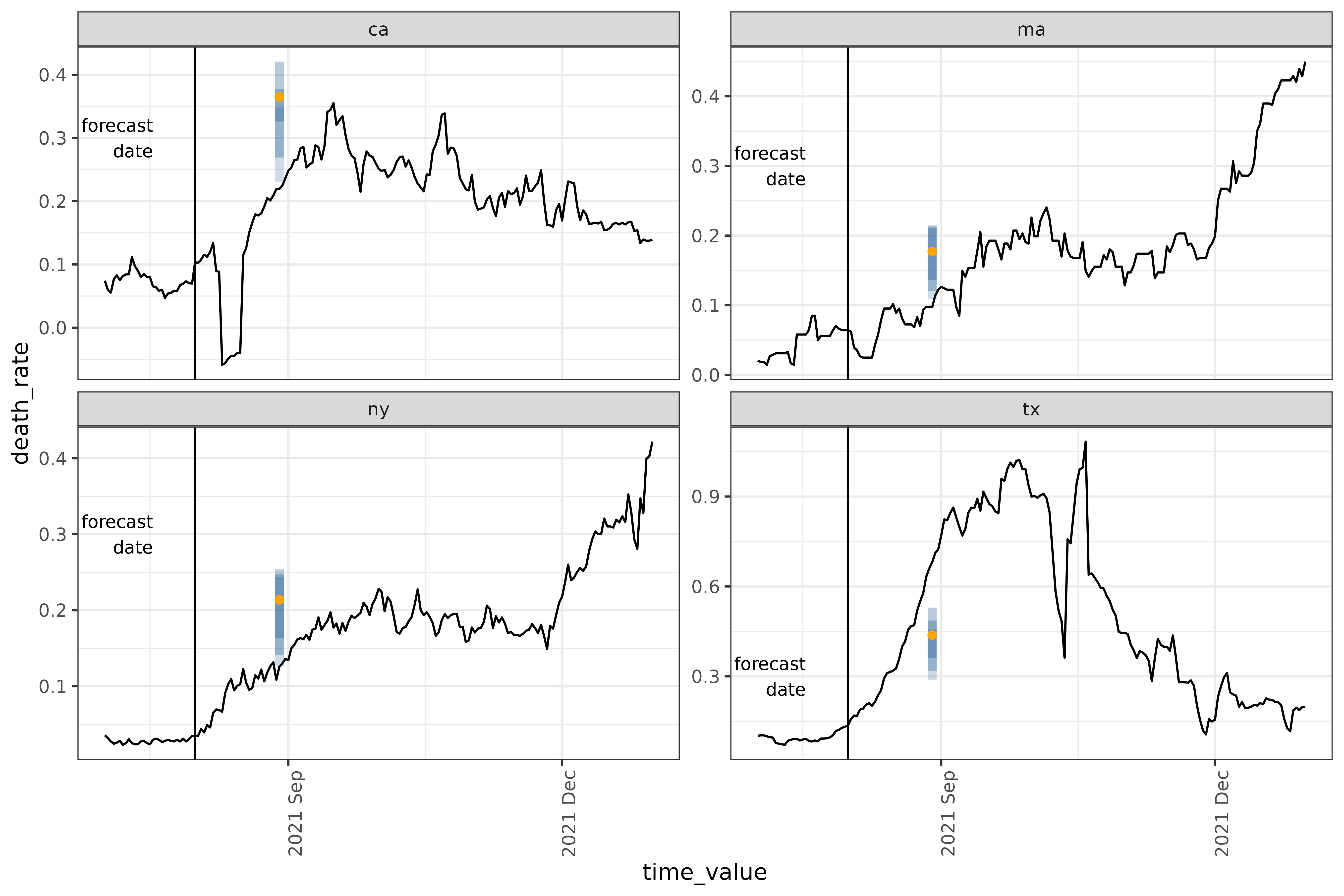

Population scaling

Suppose we want to modify our predictions to apply to counts, rather than rates. To do that, we can adjust just the frosting to perform post-processing on our existing rates forecaster. Since rates are calculated as counts per 100 000 people, we will convert back to counts by multiplying rates by the factor $\frac{regional \text{ } population}{100000}$ .

count_layers <-
  frosting() |>
  layer_predict() |>
  layer_residual_quantiles(quantile_levels = c(0.1, 0.25, 0.5, 0.75, 0.9)) |>
  layer_population_scaling(
    .pred,
    .pred_distn,
    # `df` contains scaling values for all regions; in this case it is the state populations
    df = epidatasets::state_census,
    df_pop_col = "pop",
    create_new = FALSE,
    # `rate_rescaling` gives the denominator of the existing rate predictions
    rate_rescaling = 1e5,
    by = c("geo_value" = "abbr")
  ) |>
  layer_add_forecast_date() |>
  layer_add_target_date() |>
  layer_threshold()

# building the new workflow
count_workflow <- epi_workflow(
  four_week_recipe,
  linear_reg(),
  count_layers
)
count_pred_data <- get_test_data(four_week_recipe, training_data)
count_predictions <- count_workflow |>
  fit(training_data) |>
  predict(count_pred_data)

count_predictions
#> An `epi_df` object, 4 x 6 with metadata:
#> * geo_type  = state
#> * time_type = day
#> * as_of     = 2023-03-10
#> 
#> # A tibble: 4 × 6
#>   geo_value time_value .pred .pred_distn forecast_date target_date
#>   <chr>     <date>     <dbl>   <qtls(5)> <date>        <date>     
#> 1 ca        2021-08-01 135.        [135] 2021-08-01    2021-08-29 
#> 2 ma        2021-08-01  11.3      [11.3] 2021-08-01    2021-08-29 
#> 3 ny        2021-08-01  38.2      [38.2] 2021-08-01    2021-08-29 
#> 4 tx        2021-08-01 117.        [117] 2021-08-01    2021-08-29

Custom classifier workflow

Let’s work through an example of a more complicated kind of pipeline you can build using the epipredict framework. This is a hotspot prediction model, which predicts whether case rates are increasing (up), decreasing (down) or flat (flat). The model comes from a paper by McDonald, Bien, Green, Hu et al³, and roughly serves as an extension of arx_classifier().

First, we need to add a factor version of geo_value, so that it can be used as a feature.

training_data <-
  training_data |>
  mutate(geo_value_factor = as.factor(geo_value))

Then we put together the recipe, using a combination of base {recipe} functions such as add_role() and step_dummy(), and epipredict functions such as step_growth_rate().

classifier_recipe <- epi_recipe(training_data) |>
  # Turn `time_value` into predictor
  add_role(time_value, new_role = "predictor") |>
  # Turn `geo_value_factor` into predictor
  step_dummy(geo_value_factor) |>
  # Create and lag growth rate
  step_growth_rate(case_rate, role = "none", prefix = "gr_") |>
  step_epi_lag(starts_with("gr_"), lag = c(0, 7, 14)) |>
  step_epi_ahead(starts_with("gr_"), ahead = 7, role = "none") |>
  # Divide growth rate into 3 bins.
  # Note `recipes::step_cut()` has a bug, or we could use that here.
  step_mutate(
    response = cut(
      ahead_7_gr_7_rel_change_case_rate,
      # Define bin thresholds.
      # Divide by 7 to create weekly values.
      breaks = c(-Inf, -0.2, 0.25, Inf) / 7,
      labels = c("down", "flat", "up")
    ),
    role = "outcome"
  ) |>
  # Drop unused columns.
  step_rm(has_role("none"), has_role("raw")) |>
  step_epi_naomit()

This adds as predictors:

time value (via add_role())
geo_value (via step_dummy() and the previous as.factor())
growth rate of case rate, both at prediction time (no lag), and lagged by one and two weeks

The outcome variable is created by composing several steps together. step_epi_ahead() creates a column with the growth rate one week into the future, and step_mutate() turns that column into a factor with 3 possible values,

$Z_{\ell, t}= \begin{cases} \text{up}, & \text{if}\ Y^{\Delta}_{\ell, t} > 0.25 \\ \text{down}, & \text{if}\ Y^{\Delta}_{\ell, t} < -0.20\\ \text{flat}, & \text{otherwise} \end{cases}$

where $Y^{\Delta}_{\ell, t}$ is the growth rate at location $\ell$ and time $t$ . up means that the case_rate is has increased by at least 25%, while down means it has decreased by at least 20%.

Note that in both step_growth_rate() and step_epi_ahead() we explicitly assign the role none. This is because those columns are used as intermediaries to create predictor and outcome columns. Afterwards, step_rm() drops the temporary columns, along with the original role = "raw" columns death_rate and case_rate. Both geo_value_factor and time_value are retained because their roles have been reassigned.

To fit a classification model like this, we will need to use a parsnip model that has mode = "classification". The simplest example of a parsnip classification-mode model is multinomial_reg(). We don’t need to do any post-processing, so we can skip adding layers to the epiworkflow(). So our workflow looks like:

wf <- epi_workflow(
  classifier_recipe,
  multinom_reg()
) |>
  fit(training_data)

forecast(wf) |> filter(!is.na(.pred_class))
#> An `epi_df` object, 4 x 3 with metadata:
#> * geo_type  = state
#> * time_type = day
#> * as_of     = 2023-03-10
#> 
#> # A tibble: 4 × 3
#>   geo_value time_value .pred_class
#>   <chr>     <date>     <fct>      
#> 1 ca        2021-08-01 up         
#> 2 ma        2021-08-01 up         
#> 3 ny        2021-08-01 up         
#> 4 tx        2021-08-01 up

And comparing the result with the actual growth rates at that point in time,

growth_rates <- covid_case_death_rates |>
  filter(geo_value %in% used_locations) |>
  group_by(geo_value) |>
  mutate(
    # Multiply by 7 to estimate weekly equivalents
    case_gr = growth_rate(x = time_value, y = case_rate) * 7
  ) |>
  ungroup()

growth_rates |> filter(time_value == "2021-08-01")
#> An `epi_df` object, 4 x 5 with metadata:
#> * geo_type  = state
#> * time_type = day
#> * as_of     = 2023-03-10
#> 
#> # A tibble: 4 × 5
#>   geo_value time_value case_rate death_rate case_gr
#>   <chr>     <date>         <dbl>      <dbl>   <dbl>
#> 1 ca        2021-08-01     24.9      0.103    0.356
#> 2 ma        2021-08-01      9.53     0.0642   0.484
#> 3 ny        2021-08-01     12.5      0.0347   0.504
#> 4 tx        2021-08-01     30.7      0.136    0.619

we see that they’re all significantly higher than 25% per week (36%-62%), which matches the classification model’s predictions.

See the tooling book for a more in-depth discussion of this example.

Anatomy of an epi_workflow